Tarbela reservoir monitoring using remote sensing

LCWU - Lahore, Pakistan - PHC Peridot grant

Paul Passy

2023-12-12

I - General presentation: location

Location

• Extent: 120 km² – Volume: 11.62 Gm³
• Upstream watershed: 208240 km² (≈ 25 % of the Indus basin) – Hydrological network length: 46115 km

I - General presentation: the reservoir

The Tarbela dam

• Years of construction: 1970 - 1974
• Dam height (thalweg): 148 m
• Dam length: ≈ 2.7 km
• Purpose :
  • hydro power: 234 MW, 30 % of the needs of Pakistan
  • irrigation: 50 % of total irrigation release
  • flood mitigation

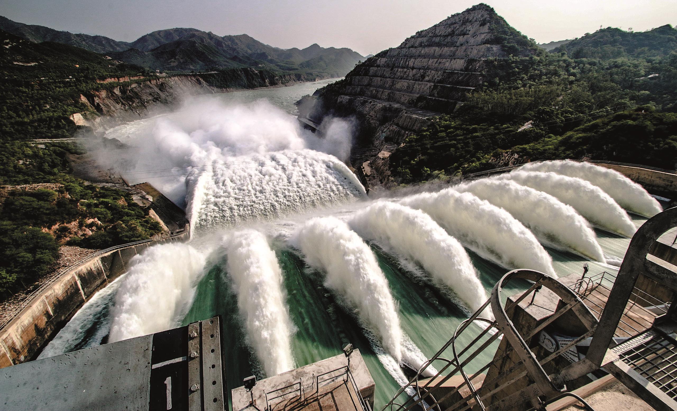
Water flowing from the Tarbela dam

I - General presentation: history

Reservoir filling

Totally filled from September 1975

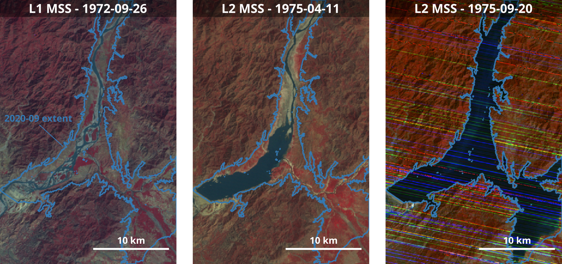
Landsat MSS false color comosites (NIR-R-G) during the filling of the reservoir

II - The issues: sedimentation

High rates of sedimentation

The reservoir has lost 30 % of its storage capacity and 15% of its power generation potential due to sedimentation (Mazhar, Mirza, Butt, et al. (2021))

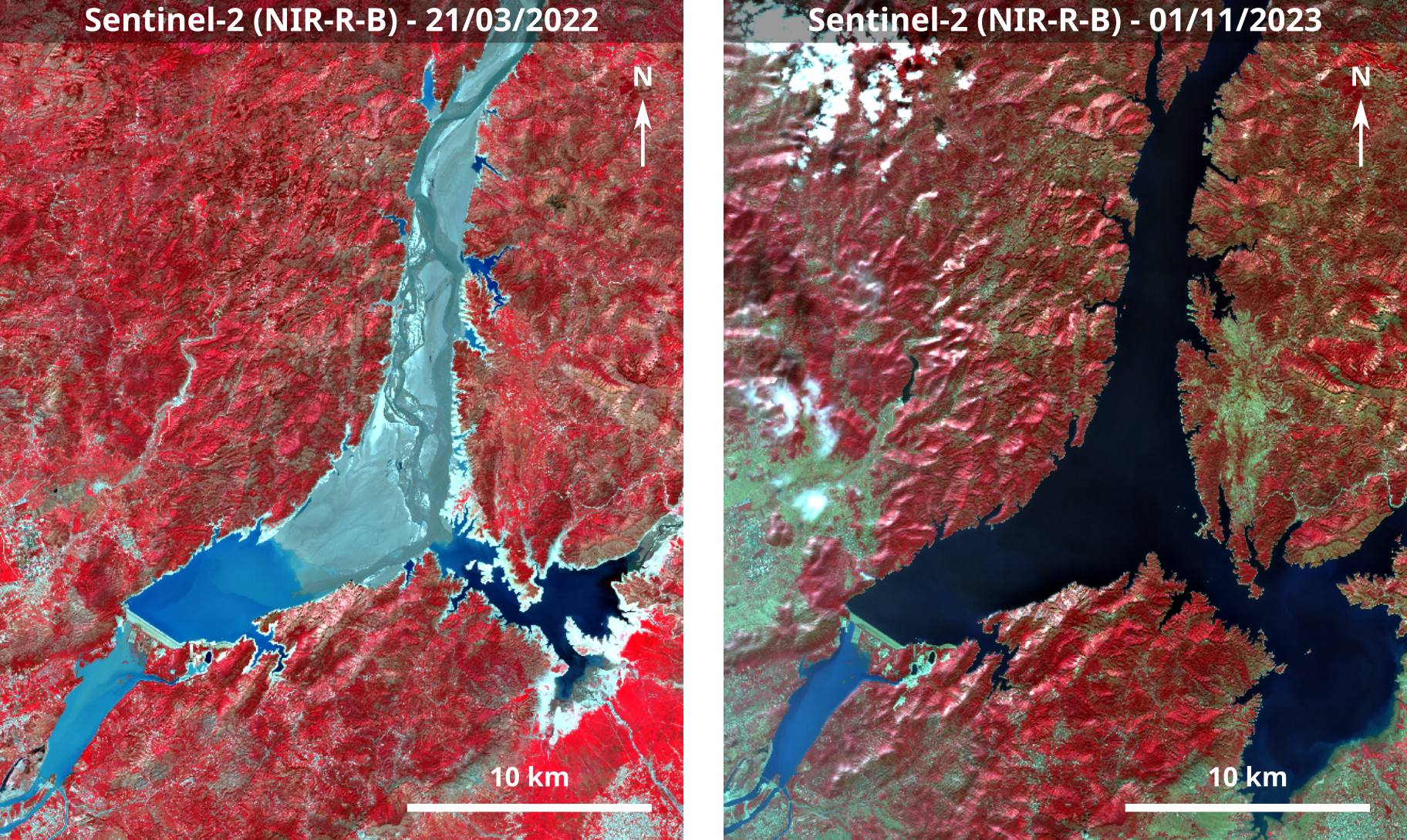
Sentinel-2 colour composites at two different dates.

II - The issues: questions

Scientific questions

• Is it possible to detect any tends in terms of water extent of the Tarbela reservoir through time?

• Is it possible to detect any tends in terms of water quality of the Tarbela reservoir through time?

• What are the links between these trends and the dynamics of the upstream watershed?

Hypothesis

• Remote sensing may help to detect the hydrological annual and pluri-annual hydrological trends

• The trends are linked to dynamics in terms of land use or climatic changes occurring within the upstream basin

III - Data: the Sentinel program

The Sentinel program

6 different missions maintained by the ESA

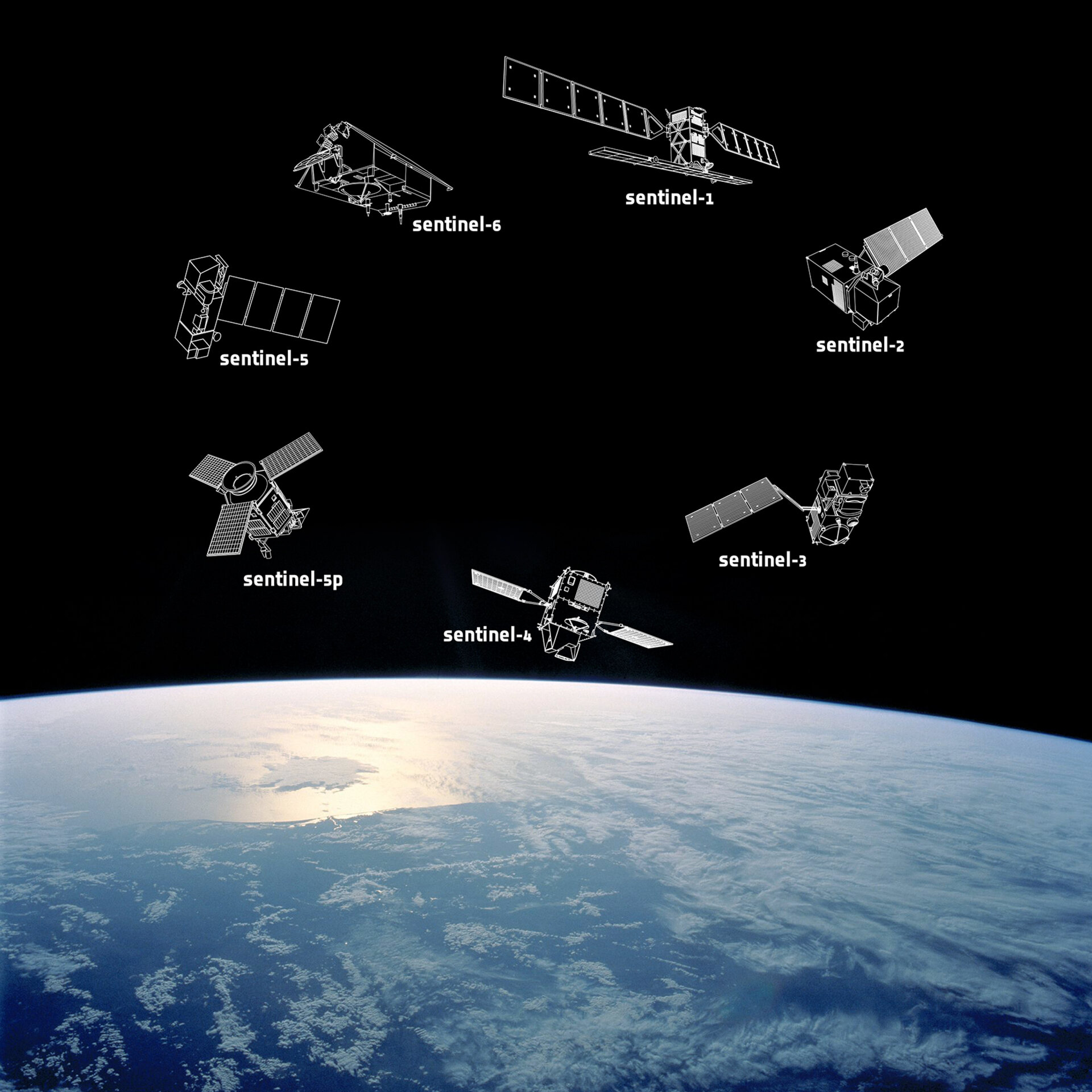
The Sentinel missions.

III - Data: Sentinel-2

The Sentinel 2 constellation

• S2 timeline
• S2 bands
• S2 revisit time
• S2 processing levels

Sentinel-2 timeline

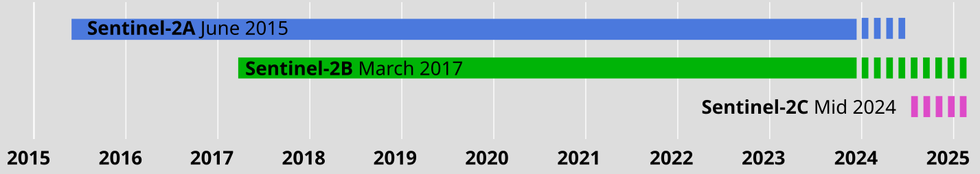
Two satellites and soon three satellites

Water flowing from the Tarbela dam

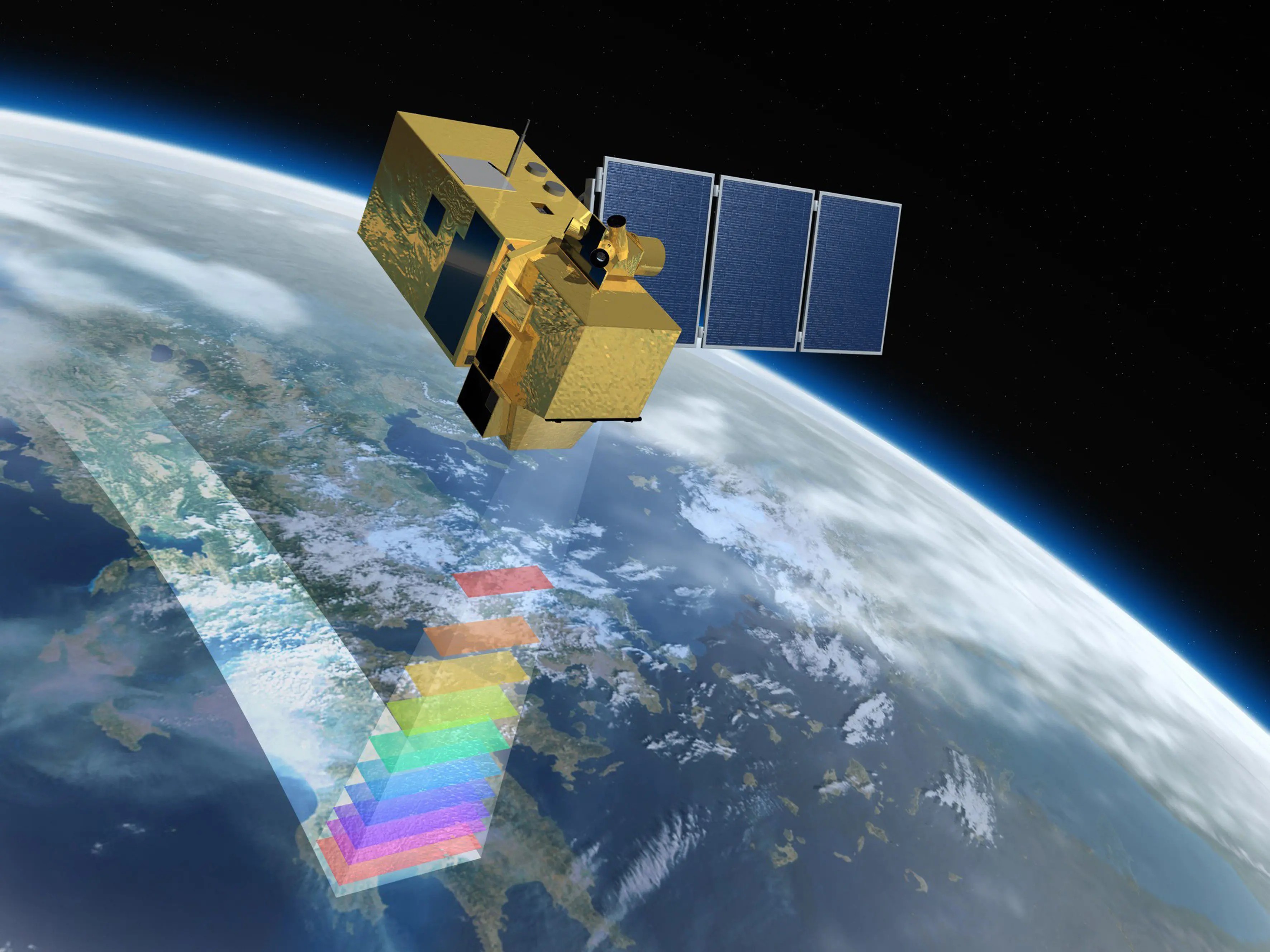
MSI sensor: 13 spectral bands

Sentinel-2 spectral bands

Band	Domain	Central l (nm)	Bandwidth(nm)	Resolution (m)
01	Coastal	442.2	21	60
02	Blue	492.1	66	10
03	Green	559.0	36	10
04	Red	664.9	31	10
05	Red Edge 1	703.8	16	20
06	Red Edge 2	739.1	15	20
07	Red Edge 3	779.7	20	20
08	NIR	832.9	106	10
8A	Narrow NIR	864.0	22	20
09	Water vapour	943.2	21	60
10	SWIR Cirrus	1376.9	30	60
11	SWIR 1	1610.4	94	20
12	SWIR 2	2185.7	185	20

• Sentinel-2A: 10 days
• Sentinel-2B: 10 days
• Sentinel-2A and 2B together: 5 days

5 days between two dates over the Tarbela reservoir

Date	Satellite
2023-10-02	Sentinel-2A
2023-10-07	Sentinel-2B
2023-10-12	Sentinel-2A
2023-10-17	Sentinel-2B
2023-10-22	Sentinel-2A
2023-10-27	Sentinel-2B
2023-11-01	Sentinel-2A
2023-11-06	Sentinel-2B
2023-11-11	Sentinel-2A
2023-11-16	Sentinel-2B
2023-11-21	Sentinel-2A

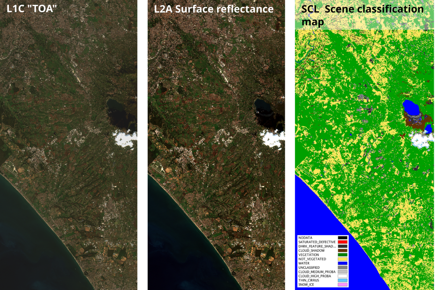
• L1C: TOA reflectance
• L2A: Surface reflectance processed using the SEN2COR algorithm

Sentinel-2 processing levels.

IV - Methods: COG

Data access

Cloud Optimized GeoTIFF: “A Cloud Optimized GeoTIFF (COG) is a regular GeoTIFF file, aimed at being hosted on a HTTP file server, with an internal organization that enables more efficient workflows on the cloud. It does this by leveraging the ability of clients issuing HTTP GET range requests to ask for just the parts of a file they need.”

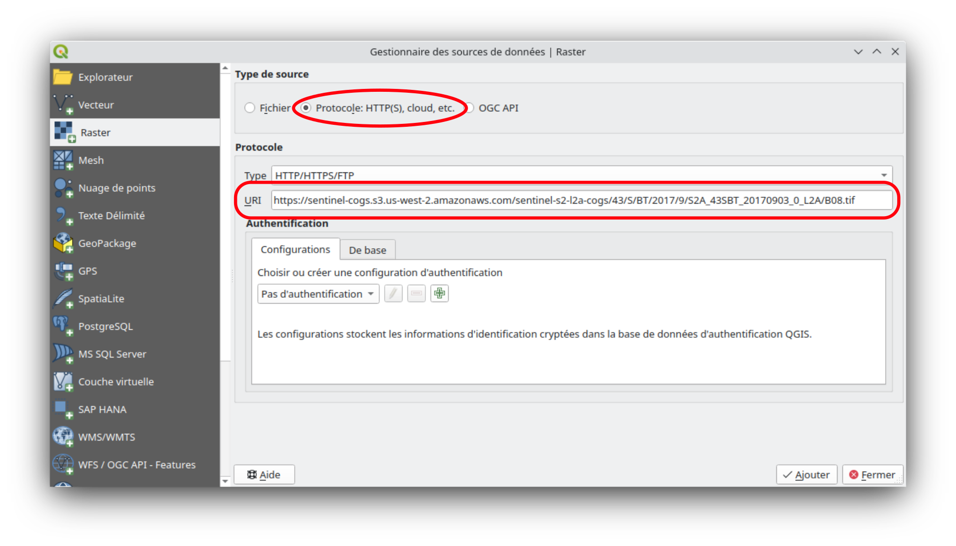
COG in QGIS.

IV - Methods: clouds

Clouds survey

Calculation of clouds proportion only on the study area

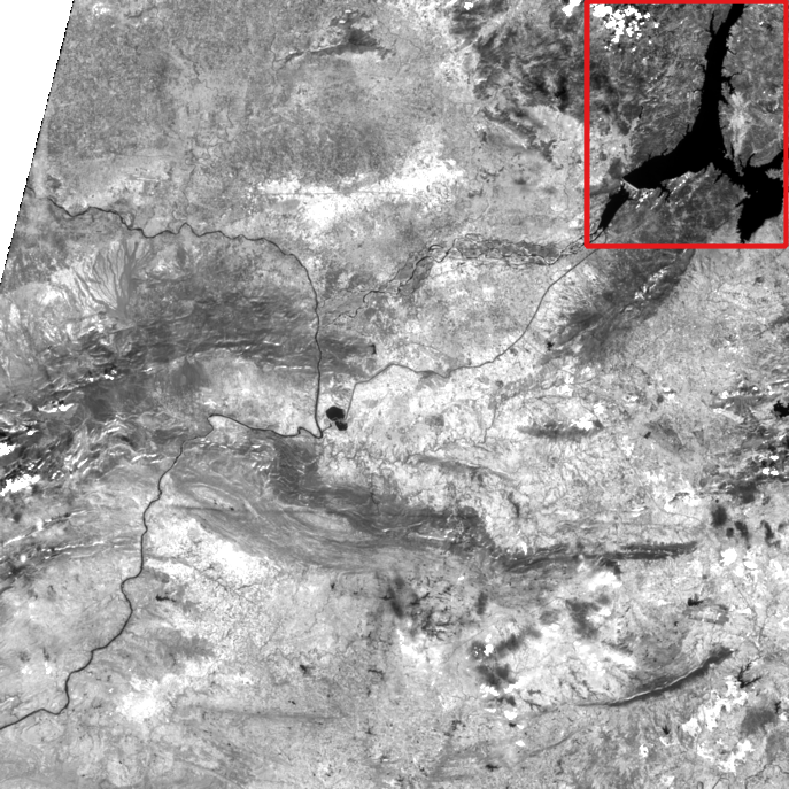
Sentinel-2 tile T43SBT and the study area (red).

Cloud cover over the whole tile (as provided in the metadata of the image): 15 %

IV - Methods

Clouds survey

Calculation of clouds proportion only on the study area

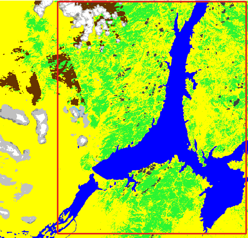
SCL raster for the study area

Cloud cover over the study area (as calculated using the SCL raster): 9 %

IV - Methods: clouds chronics

Chronics of cloud cover

Cloud cover the study area for the whole chronics (01-2017 - 11-2023)

IV - Methods: cloud cover by month

Cloud cover by month

Cloud cover the study area by month (01-2017 - 11-2023)

High proportion of clouds in January.

IV - Methods: algorithm

Water detection

The chosen algorithm: the Python package WaterDetect (Cordeiro, Martinez, and Peña-Luque (2021))

Advantages:

• automatic threshold for water detection (useful for temporal analysis)
• very few False Positive water pixels
• remove not pure water pixels (shores are excluded)

IV - Methods: effect of the algorithm

WaterDetect VS MNDWI VS AWEI

Example for the 2022-04-10 comparing WaterDetect and the MNDWI (Feyisa et al. (2014))

WaterDetect is spatially more precise.

IV - Methods: effect on the water mask

Implications of the choice of the water mask

Direct impacts of the water mask in the water quality parameters calculations.

IV - Methods: water quality from space

The water quality is linked to the water colour

The suspended and dissolved matters change the colour of water and thus its spectral signature.

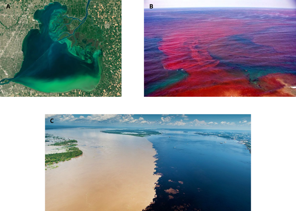
A) “Green waters” Algal bloom, B) “Red waters” Harmful algae bloom, C) Rio Negro - Amazon confluence

IV - Methods: signal inversion

Signal inversion of the Sentinel-2 reflectances to obtain water quality parameters

• SPM
• Turbidity
• Chlorophyl-a
• CDOM

SPM: Suspended Particulate Matter

According to Nechad (Nechad, Ruddick, and Park (2010))

\[ spm = a \times \frac{Red}{(1 - \frac{Red}{c})} \]

with:

• Red: the reflectance in the Red band
• a: 610.94
• c: 0.2324

High concentrations of SPM may reflect high rates of erosion in the upstream watershed.

According to Dogliotti (Dogliotti et al. (2015))

    """Switching semi-analytical-algorithm computes turbidity from red and NIR band

    following Dogliotti et al., 2015
    :param water_mask: mask with the water pixels (value=1)
    :param rho_red : surface Reflectances Red  band [dl]
    :param rho_nir: surface Reflectances  NIR band [dl]
    :return: turbidity in FNU
    """

    limit_inf, limit_sup = 0.05, 0.07
    a_low, c_low = 228.1, 0.1641
    a_high, c_high = 3078.9, 0.2112

    t_low = nechad(Red, a_low, c_low)
    t_high = nechad(Nir2, a_high, c_high)
    w = (Red - limit_inf) / (limit_sup - limit_inf)
    t_mixing = (1 - w) * t_low + w * t_high

    t_low[Red >= limit_sup] = t_high[Red >= limit_sup]
    t_low[(Red >= limit_inf) & (Red < limit_sup)] = t_mixing[(Red >= limit_inf) & (Red < limit_sup)]
    t_low[t_low > 4000] = 0
    return t_low

with:

• Red: the reflectance in the Red band
• Nir: the reflectance in the NIR band

High turbidity may reflect high rates of erosion in the upstream watershed or high algal productivity within the water column.

According to Gitelson and Kondratyev, 1991

\[ chl = 61.324 \times \frac{RedEdge1}{Red} - 37.94 \]

with:

• Red: the reflectance in the Red band
• RedEdge1: the reflectance in the Red edge 1 band

High concentrations of chlorophyll reflects high algal productivity and maybe high loads of nutrients.

CDOM: Colored dissolved organic matter is the optically measurable component of dissolved organic matter in water.

According to Brezonik (Brezonik et al. (2015))

\[ cdom = \exp(1.872 - 0.830 \times \log(\frac{Blue}{RedEdge2})) \]

High concentrations of CDOM may reflect high loads of dissolved organic matter from the watershed.

IV - Methods: let’s recap

The chain of treatments

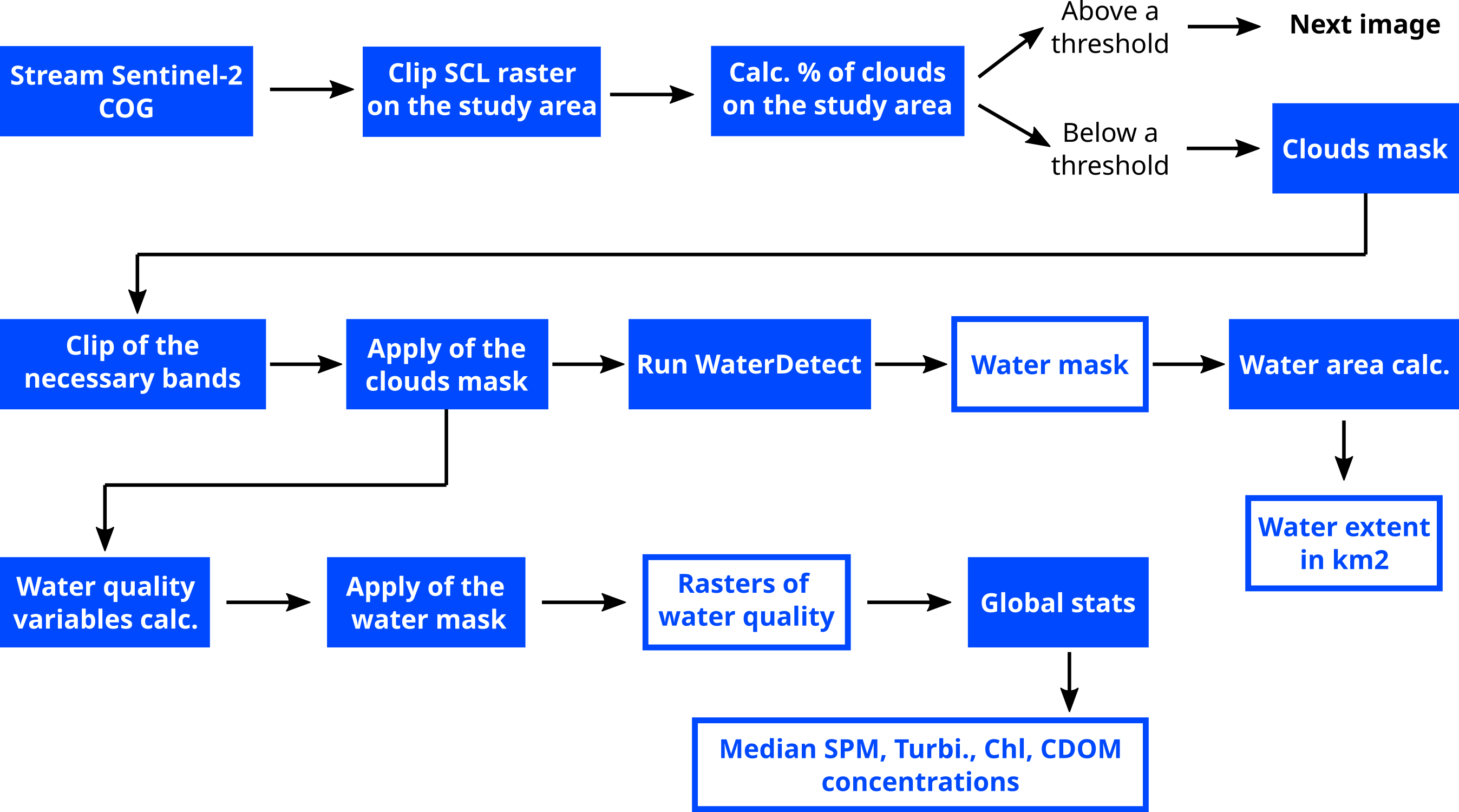
The global chain of treatments

V - Results: chronics of water extents

Water extents on the whole period

High intra-annual variations.

V - Results: water extents by year

Water extents by year

On average the extents were the highest in 2020.

Minimum values need to be manually checked!

V - Results: water extents by month

Water extents by month

Min extent → March - Max extent → August

V - Results: chronics of SPM

Chronics of SPM (2017 - 2023)

• SPM chronics
• SPM by year
• SPM by month

Median SPM concentrations by year

Less SPM in 2020.

Median SPM concentrations by month

Max SPM → June - Min SPM → December.

V - Results: chronics of turbidity

Chronics of turbidity (2017 - 2023)

• Turbidity chronics
• Turbidity by year
• Turbidity by month

Median turbidity by year

Less turbidity in 2020.

Median turbidity by month

Max turbidity → June - Min SPM → December.

V - Results: chronics of Chlorophyll

Chronics of chlorophyll (2017 - 2023)

• Chlorophyll chronics
• Chlorophyll by year
• Chlorophyll by month

Median chlorophyll concentrations by year

No clear trends for chlorophyll.

Median chlorophyll concentrations by month

Max chlorophyll → September - Min chlorophyll → December.

V - Results: chronics of CDOM

Chronics of CDOM (2017 - 2023)

• CDOM chronics
• CDOM by year
• CDOM by month

CDOM median by year

No clear trends for CDOM

CDOM median by month

Two peaks for CDOM → June and October.

V - Results: correlations

Correlation between water extents and water quality parameters

What are the links between the water extents and the variations in terms of water quality?

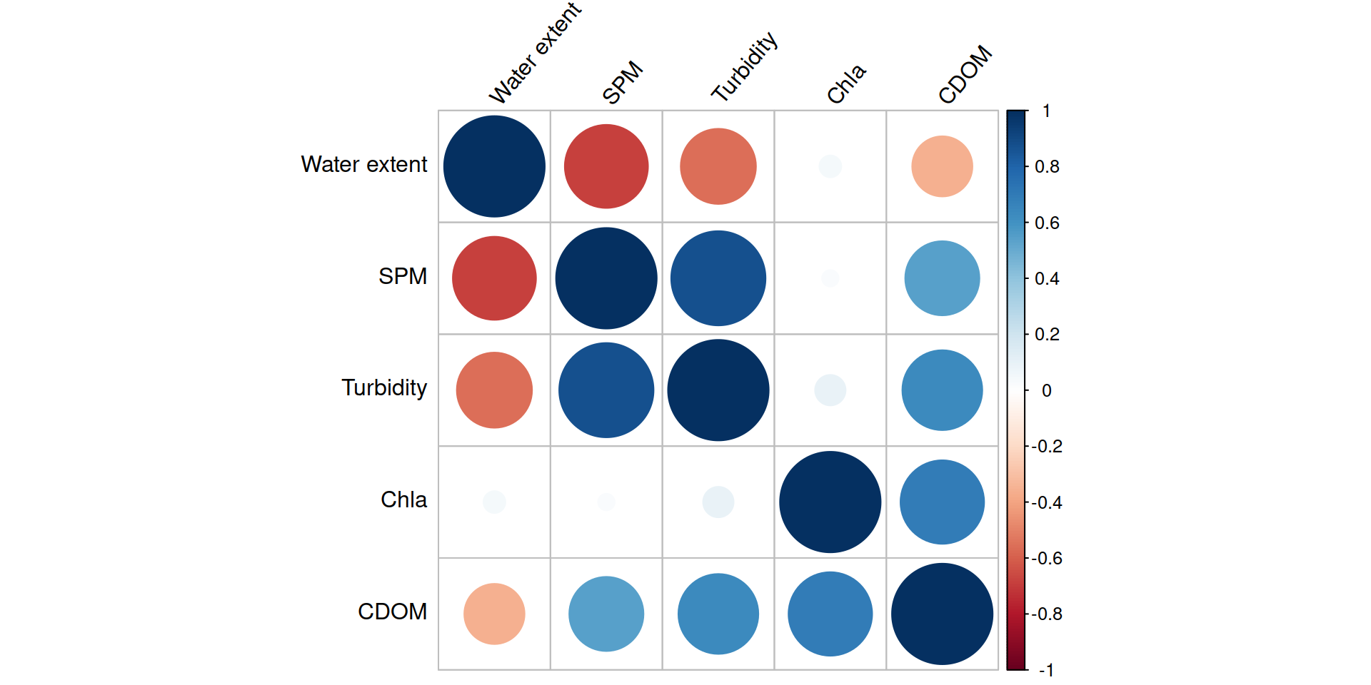
• Low water extents: large SPM, Turbidity and CDOM concentrations
• Large water extents: low SPM, Turbidity and CDOM concentrations
• Chlorophyll is not correlated to any other parameter

V - Results: water quality mapping

Spatio-temporal variations of the water quality

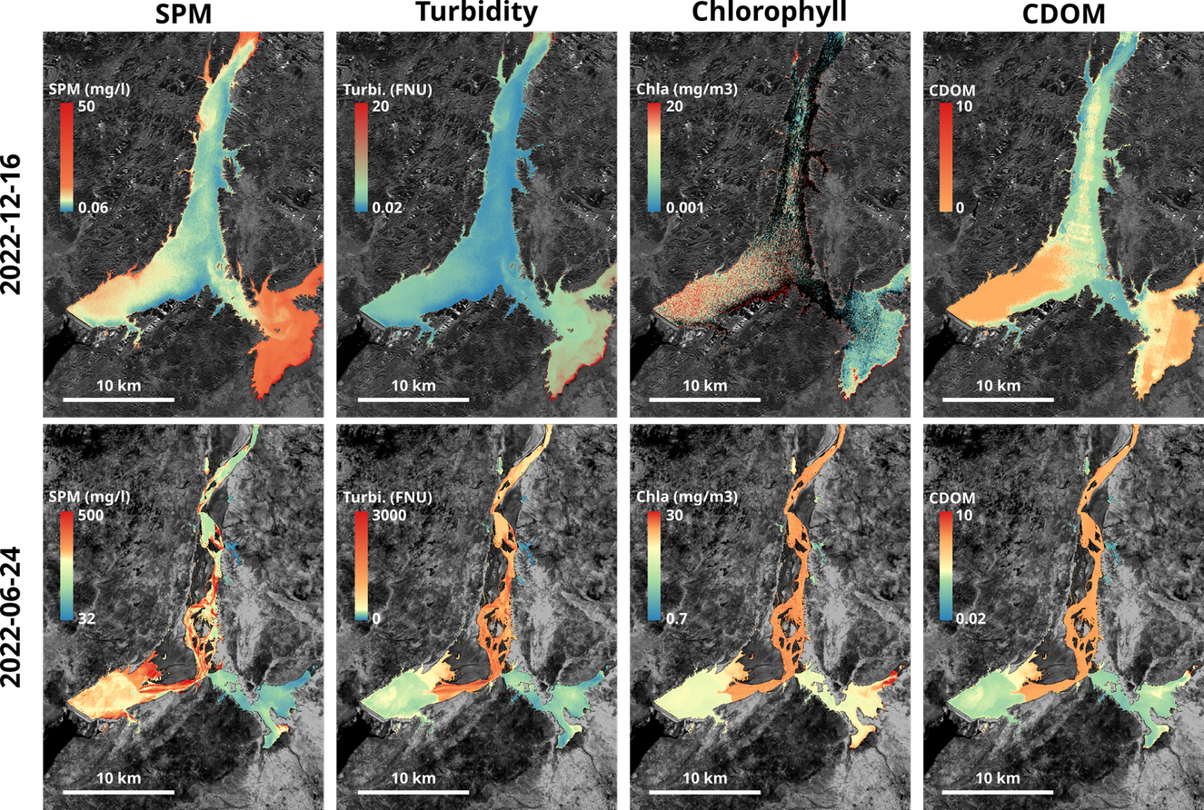
Water quality for June and December 2020

High intra-annual variability

V - Limits and perspectives

Limits

• In some cases the WaterDetect algorithm does not detect all the water
• Comparison with in-situ measurements

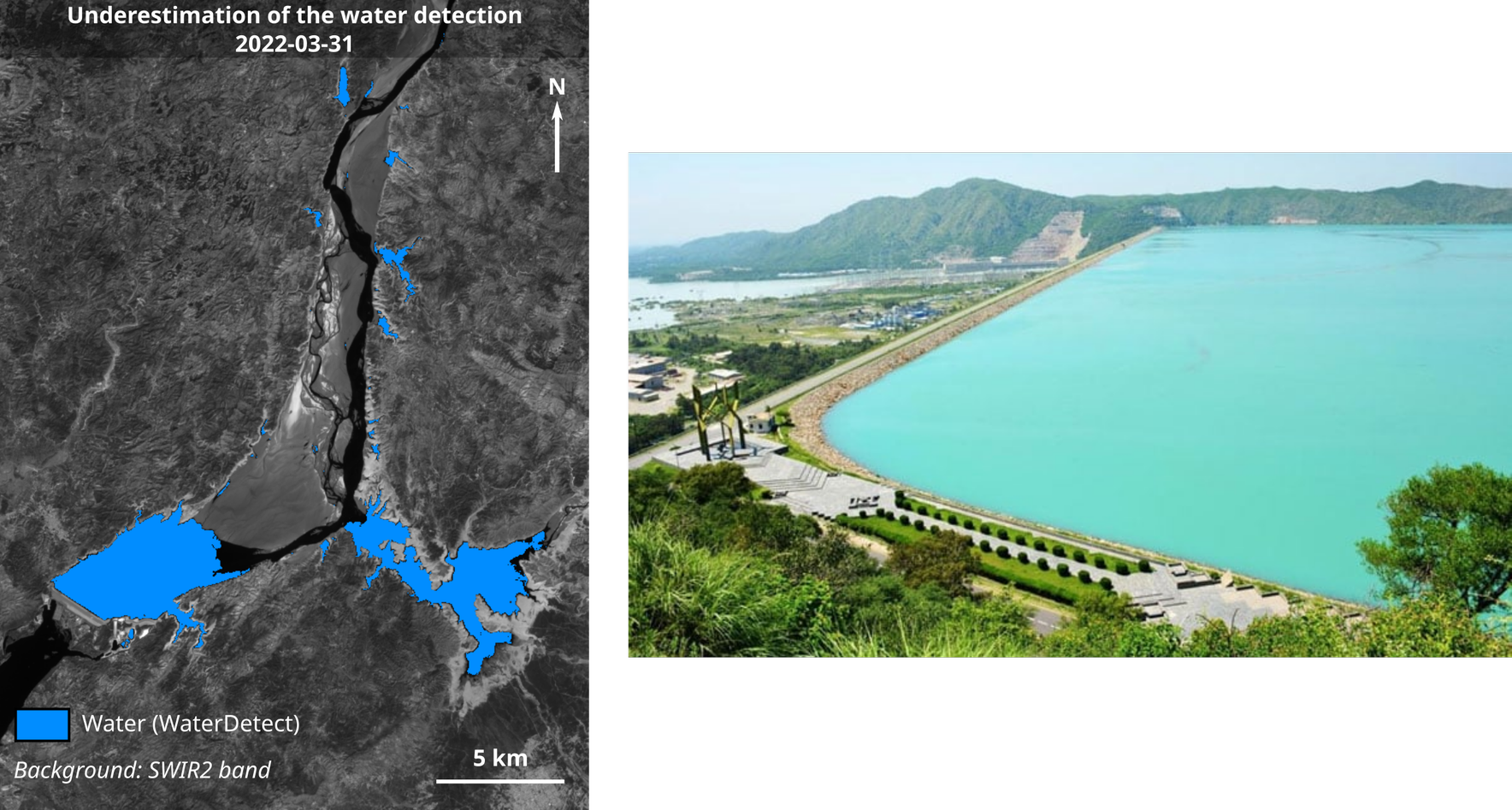
Under estimation of the WaterDetect algorithm and in-situ measurements

V - Limits and perspectives

Perspectives

Concerning the Tarbela reservoir monitoring

• Consolidate the results (check the water detection for different dates)
• Explore a longer chronics using the Landsat archives (water quality mapping issues?) (Maciel et al. (2023))

Concerning the upstream watershed

Link the hydrological trends with dynamics of the upstream watershed as:

• precipitations / temperatures changes (Mazhar, Mirza, Abbas, et al. (2021))
• land cover/land use changes
• vegetation changes
• snow cover changes (Gascoin (2021))
• … other changes?

Glaciers melting in Himalaya

V - Conclusion

• we developed an automatic treatment chain to survey the Tarbela reservoir from Sentinel-2 images
• 158 Sentinel-2 images were treated from 2017-03-27 to 2023-11-16
• we highlighted trends in terms of water extents
  • at the scale of one year: min extent in March and max extent in August
  • at the scale of the period: largest extent in 2020 and smallest extent in 2018
• we highlighted trends in terms of water quality variations
  • at the scale of one year:
    • SPM and turbidity max in June
    • SPM and turbidity min in December
    • CDOM shows two peaks in the year in June and in October
  • at the scale of the period:
    • SPM and turbidity are lower in 2020
    • chlorophyll and CDOM seem to be more stable through time

شکریہ

References

Brezonik, Patrick L., Leif G. Olmanson, Jacques C. Finlay, and Marvin E. Bauer. 2015. “Factors Affecting the Measurement of CDOM by Remote Sensing of Optically Complex Inland Waters.” Remote Sensing of Environment, Special issue: Remote sensing of inland waters, 157 (February): 199–215. https://doi.org/10.1016/j.rse.2014.04.033.

Cordeiro, Maurício C. R., Jean-Michel Martinez, and Santiago Peña-Luque. 2021. “Automatic Water Detection from Multidimensional Hierarchical Clustering for Sentinel-2 Images and a Comparison with Level 2A Processors.” Remote Sensing of Environment 253 (February): 112209. https://doi.org/10.1016/j.rse.2020.112209.

Dogliotti, A. I., K. G. Ruddick, B. Nechad, D. Doxaran, and E. Knaeps. 2015. “A Single Algorithm to Retrieve Turbidity from Remotely-Sensed Data in All Coastal and Estuarine Waters.” Remote Sensing of Environment 156 (January): 157–68. https://doi.org/10.1016/j.rse.2014.09.020.

Feyisa, Gudina L., Henrik Meilby, Rasmus Fensholt, and Simon R. Proud. 2014. “Automated Water Extraction Index: A New Technique for Surface Water Mapping Using Landsat Imagery.” Remote Sensing of Environment 140 (January): 23–35. https://doi.org/10.1016/j.rse.2013.08.029.

Gascoin, Simon. 2021. “Snowmelt and Snow Sublimation in the Indus Basin.” Water 13 (19): 2621. https://doi.org/10.3390/w13192621.

Maciel, Daniel Andrade, Nima Pahlevan, Claudio Clemente Faria Barbosa, Evlyn Márcia Leão de Moraes de Novo, Rejane Souza Paulino, Vitor Souza Martins, Eric Vermote, and Christopher J. Crawford. 2023. “Validity of the Landsat Surface Reflectance Archive for Aquatic Science: Implications for Cloud-Based Analysis.” Limnology and Oceanography Letters 8 (6): 850–58. https://doi.org/10.1002/lol2.10344.

Mazhar, Nausheen, Ali Iqtadar Mirza, Sohail Abbas, Muhammad Ameer Nawaz Akram, Muhammad Ali, and Kanwal Javid. 2021. “Effects of Climatic Factors on the Sedimentation Trends of Tarbela Reservoir, Pakistan.” SN Applied Sciences 3 (1): 122. https://doi.org/10.1007/s42452-020-04137-4.

Mazhar, Nausheen, Ali Iqtadar Mirza, Zayanah Sohail Butt, Muhammad Nawaz, and Muhammad Ameer Nawaz Akram. 2021. “Advancement of the Pivot Point of Underwater Delta: A Study of Tarbela Reservoir, Haripur, Pakistan.” Journal of Himalayan Earth Sciences 54 (2): 40–46.

Nechad, B., K. G. Ruddick, and Y. Park. 2010. “Calibration and Validation of a Generic Multisensor Algorithm for Mapping of Total Suspended Matter in Turbid Waters.” Remote Sensing of Environment 114 (4): 854–66. https://doi.org/10.1016/j.rse.2009.11.022.